Language Identification using NLTK
Most of us are used to search engines such as Google or Bing offering us translation services when we reach a page in a foreign language. For instance, you might have noticed this translation popup in Google’s Chrome browser before:
![]()
I was curious how this mechanism worked and how I could use it in my own projects. So, if you’re working on a search engine of your own, developing another tool that requires language detection, or simply curious like me, continue reading.
Initial thoughts
The most obvious programmatic approach that came to mind was a dictionary comparison with the words from the sample text. Look up each word from the sample text in dictionaries for different languages, the more matches between a sample and a specific dictionary, the more likely it is to belong to that language. The equally obvious drawback is the need to compile language-representative dictionaries and store them. However, this isn’t a large drawback for two reasons: first, these days, storage is relatively cheap, and second, Google reports that approximately 50 languages cover nearly all web content, so at most you would need just those language dictionaries.
The real problem with this approach is that even within that relatively small group of languages, some are highly inflected and closely related. So while the roots of words remain relatively stable, their inflections change depending on what job the word is doing in the sample text, and this can complicate naive match attempts to a dictionary. Furthermore, we should consider the source of the sample text may be the result of Automatic Speech Recognition (ASR) or Optical Character Recognition (OCR) processing. One should expect a fair number of transcription errors. Here, as well, a brute-force dictionary comparison would likely struggle and have an unacceptable error rate.
So what’s a better way? Well, there are several interesting approaches of varying complexity and accuracy, some depend on the type of input and data you have. I’m going to start with a method called “TextCat” in this post and show a few other methods in future posts, including the one Google actually uses. The concepts discussed here will be useful for understanding future posts.
I assume that you’ve already installed Python and NLTK for the remainder of the post.
N-Grams
An N-gram is a contiguous N-character chunk of a longer string. N-grams are generated in a “sliding window” fashion so that multiple N-grams of a single string share overlapping characters. In many NLP applications the blanks before and after the word are also represented, we will use the “<” character to denote the blank before a word and “>” for the blank after.
Common N-gram patterns are often named; a pattern of 2-character chunks is called a bi-gram, 3-characters, tri-gram, and so on. Generally speaking, bigrams and trigrams are the ones you’ll deal with most often because it turns out training ML models on more than a trigram often results in too much data sparsity.
NLTK has an N-gram module so let’s use that with the word “Python” as an example:
# Import the N-gram module
from nltk.util import ngrams

# Some useful definitions
START_CHAR = "<"
END_CHAR = ">"
word = "Python"
full_word = START_CHAR + word + END_CHAR

# Generate bigrams
bigrams = ngrams(list(full_word), 2)
for gram in bigrams:
    print(gram)

# Will output:
('<', 'P')
('P', 'y')
('y', 't')
('t', 'h')
('h', 'o')
('o', 'n')
('n', '>')
NLTK also has convenience methods bigrams() and trigrams() we could use directly:
trigrams = trigrams(list(full_word))
for gram in trigrams:
    print(gram)

# Outputs:
('<', 'P', 'y')
('P', 'y', 't')
('y', 't', 'h')
('t', 'h', 'o')
('h', 'o', 'n')
('o', 'n', '>')
Zipf’s Law
You’ve probably heard about letter frequency distributions before, the observation that most languages have a characteristic distribution of letters which is strongly apparent in longer texts. For instance, you can find a break down of modern English letter frequencies here.
Letter frequencies are used in cryptanalysis and have had a strong influence on the design of the modern QWERTY keyboard. A more familiar example might be the game show Wheel of Fortune.
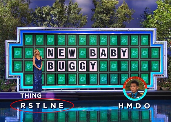
The reason the letters R, S, T, L, N, E are given for “free” to contestants during the final puzzle round is that historically they were most frequently chosen in the early years of the show, when the finalist was only allowed to choose 5 consonants and a vowel. Contestants either studied letter frequencies or intuitively understood them through game play or fluency in English. Obviously you would expect RSTLNE to show up rather sparsely in final puzzles today as a result, which is indeed the case, as opposed to regular rounds where the letters appear with expected frequency. There’s an interesting analysis of this over at Slate.
It turns out a similar phenomenon holds true not just for letters but for words as well. To show this, during the 1940’s American professor George Kingsley Zipf actually paid a room full of people to count words in newspapers and periodicals. In fact, it turns out words, phrases, and whole sentences of a language seem to share this frequency pattern.
Although this regularity was observed prior to his efforts it was Zipf who popularized the idea before his untimely death at the age of 48. Hence this empirical rule is known as Zipf’s Law and the shape of the resulting curve when graphed is a “Zipf curve” for that text. If you were to transform a Zipf curve graph using log-log scale it would appear as a straight line with a slope of -1.
For a sense of how profound this observation is consider that about half of the famous Brown Corpus, totalling roughly 1 million words, can be covered by only 135 words when you measure word-count frequency! In fact, it might surprise you to learn that only 10 words account for 25% of the English language.
Don’t believe it? Take a look at a cumulative frequency graph for 50 top words in Moby Dick:
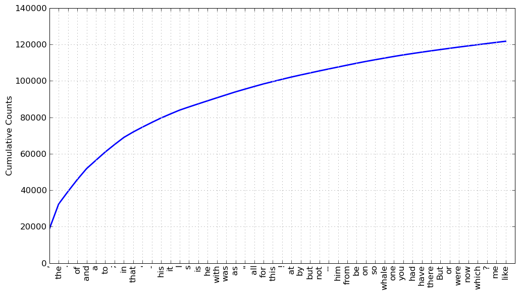
Cumulative frequency graph for 50 top words in Moby Dick
The top 50 words account for almost half of all the words in the book! What’s fascinating about Zipf’s Law is that it holds up for most languages and nobody really knows why. You might object that this is simply the magic of power laws but consider studies such as ones done by Wentian Li, where he demonstrates that words generated by randomly combining letters still create a Zipf curve, it’s not obvious why this should be true. You can read more about that in the paper Random texts exhibit Zipf’s-law-like word frequency distribution.
To get a feel of everything we’ve been talking about so far try to play around with the code below, using different input texts:
import urllib2
import html2text
import regex
import nltk
from nltk.util import trigrams
from nltk.probability import FreqDist
from nltk.tokenize import word_tokenize

def clean_text(text):
    clean = regex.sub(r"[^\P{P}\']+", "", text)
	             .replace('\n', ' ')
                 .replace('\r', ' ')

    return html2text.html2text(clean)

# The Great Gatsby
url = 'http://gutenberg.net.au/ebooks02/0200041.txt'
response = urllib2.urlopen(url).read().decode('latin-1')
tokens = word_tokenize(clean_text(response))

profile = FreqDist()
for t in tokens:
    token_trigrams = trigrams(list(t))

    # Build our profile
    for cur_trigram in token_trigrams:
        # If we've encountered it before, just increment by 1
        if cur_trigram in profile:
            profile[cur_trigram] += 1
        else:
            # First encounter, set count to 1
            profile[cur_trigram] = 1

# Print some stats
most_common = profile.most_common(10)
for w in most_common:
    print(''.join(w[0]) + ': ' + str(w[1]))
The above is aimed at Python 2.7, you’ll need to install urllib2, html2text, and regex (module that supports Unicode codepoint properties with the \p{} syntax). The code first grabs the full text for the novel “The Great Gatsby” from Project Gutenberg, converts HTML to pure text, removes newline, carriage return characters, and all punctuation except apostrophes. Second, tokenize the text and iterate over the tokens to generate trigrams, breaking each word up into smaller pieces. Finally, we count how often we encounter each piece in the entire novel.
In the end, your output should be:
the: 3075
and: 1792
ing: 1499
her: 1051
was: 820
hat: 817
ere: 764
his: 661
tha: 634
ent: 577
Although this isn’t a large corpus of text we can immediately recognise the top few words as being in line with our intuition about most common English words.
TextCat
So what do N-grams and professors with cool last names have to do with language identification? Well, we’ve already seen that we can use N-grams to analyze text in smaller pieces than a word and that Zipf’s Law explains how languages have characteristic curves. In 1994 William B. Cavnar and John M. Trenkle observed that Zipf’s Law holds true for N-grams as well. What was true of the whole word is true of its parts.
Cavnar and Trenkle came up with a text categorization algorithm that exploits this. Although it is by no means new-or even that advanced-it is quite effective. It’s main advantages are simplicity, speed, and ability to use in contexts other than language identification such as categorising documents.
The original algorithm is described in “N-Gram-Based Text Categorization”, also known as “Text Cat”.
TextCat is a supervised learning method that relies on first using representative samples of languages to create profile for them. It does this by generating a ranked (sorted most frequent to least) list of unique N-grams, then for any input text to be classified, you perform the same profiling and measure “closeness” between the language and sample profiles.
To train our language identifier we must do something similar to the sample code provided for analyzing N-grams for The Great Gatsby, generating profiles for all the languages we’re interested in. In the example above we were able to easily use a freely available corpus of text (the novel), but in practice we must gather a lot more information than this for each language. This can be a difficult task because there are many languages, dialects, many are under represented, and finding reliable sources for them can be quite time consuming.
I used data from a project designed to solve this problem, it’s maintained by Alex Rudnick and makes available a directory of trigram frequencies for many writing systems using a web crawler called “An Crubadan”.
The web crawler works at the level of “writing systems” rather than “languages”, so that Serbian Cyrillic and Serbian Latin are treated separately. The key advantage of this web crawler is that it has representation for lesser-known languages, ones that may not have easy representative samples online through resources such as Wikipedia. Notably missing from this data set are Japanese and Chinese.
The data made available by the web crawler is obviously much larger than the toy example above with The Great Gatsby, for comparison’s sake, take a look at the top trigrams for English (remember “<” means space before word, and “>” after):
954187 <th
728135 the
655273 he>
360758 ing
359481 nd>
351373 ng>
345633 <an
333091 <to
329517 ed>
316431 <of
312505 and
309917 to>
297557 of>
...
First, note there are 728135 instances of the word “the” in the web crawler’s corpus versus our novel with only 3075. In spite of being encountered almost 240 times more rank is roughly preserved. You can see a lot of other similarities between the two lists and it’s exactly this property that we’re going to exploit. In practice, it turns out you don’t need that much sample text as the N-gram profiles are remarkably consistent, although there are limits on how short a sample can be.
I wrote a corpus reader to process trigram files provided by the Crubadan project using NLTK’s set of modules to aid in the task of profiling. The reader simply processes all the language trigram files and creates frequency distributions based on them as well as provides some helper functions to map between Crubadan codes to ISO 639-3 codes. I’ll skip this part as it’s not directly related to the language detection algorithm itself.
So, given a random piece of text, how do we guess what language it is? As before, first remove all punctuation from our sample (except apostrophes) and tokenize using NLTK’s word_tokenize() function. Then generate trigrams for each token and keep track of the number of times we encounter each trigram, this is our “sample profile”.
def remove_punctuation(self, text):
    return re.sub(r"[^\P{P}\']+", "", text)

clean_text = remove_punctuation(text)
tokens = word_tokenize(clean_text)
Now, let’s create a “fingerprint” of the cleaned sample text:
# Our frequency distribution object
fingerprint = FreqDist()
# Loop through all our words
for t in tokens:
    # Generate trigrams for each word
    token_trigrams = self.trigrams(t)
    # Count each trigram
    for cur_trigram in token_trigrams:
        # If we've encountered it before, just increment by 1
        if cur_trigram in fingerprint:
            fingerprint[cur_trigram] += 1
        else:
            # First encounter, set count to 1
            fingerprint[cur_trigram] = 1
Here’s the important part: the TextCat algorithm calculates the “closeness” between each language and the profile sample by using an intuitive metric it calls the “out-of-place” measure. The out-of-place measure is a simple rank statistic calculating how far out of place a trigram in one profile is from itself in a second profile. Here’s the illustration from the original paper:
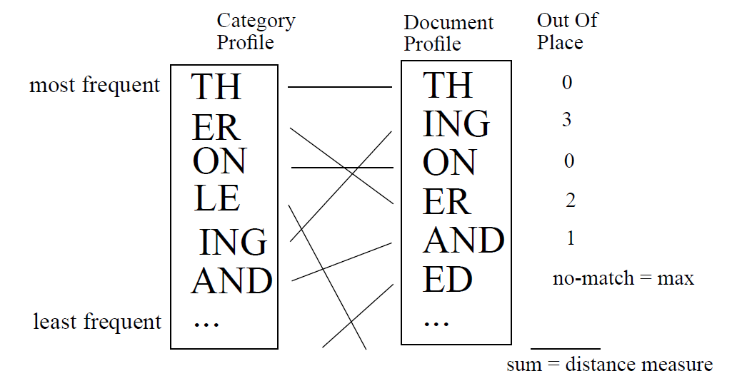
Distance measure from original paper
On the left side we see the box “Category Profile” (more on this later), this is actually our language profile. The trigrams in the box represent the frequency distribution from most frequent to least - “TH>” being the most frequent in English. On the right side we see the box marked “Document Profile” which refers to any input text whose language we’re attempting to identify. This profile is generated exactly the same way the language profile was.
On the far right of the above image we see the out-of-place measure, since “TH>” has highest rank in both the language and sample profile, their “distance” is 0. In contrast, the trigram “ER>” has rank 2 in the language profile but rank 4 in the sample profile, for a distance of 2. If you repeat this calculation for all trigrams and sum the individual distances you’ll get an overall distance measure between the language and sample.
If we run across a trigram in the sample that is not in the language profile we penalize this by adding a large number to the sum. This is because we expect to have well over 90% coverage for our language profiles (see Zipf’s Law section above for why), not finding a trigram in a profile is extremely unlikely and probably means this isn’t the correct language.
Let’s see how this plays out in code, assume the frequency distribution for English is stored in the variable “lang_fd” and the frequency distribution for our sample text is stored in the variable “text_profile”. Here’s how we’d calculate the out-of-place measure:
dist = 0
# Is this trigram in the FreqDist of this language at all?
if trigram in lang_fd:
    # Get index into FreqDist for language
    idx_lang_profile = lang_fd.keys().index(trigram)
    # Get index into FreqDist for sample
    idx_text = text_profile.keys().index(trigram)

    # Calculate the distance between them
    dist = abs(idx_lang_profile - idx_text)
else:
    # This trigram isn't in the language's profile
    # Penalize this heavily by adding max int
    dist = maxint
Performing the above for each language, keeping track of “dist”, we will end up with a dictionary of languages and their corresponding distance to the sample text. The smallest distance will most likely correspond to the associated language.
Conclusion
I started this post by pointing out Google’s language detection capability in Chrome. Although the technique I described works very well, and in fact is in use by some commercial projects (eg: GATE), it’s not how Google does it.
Richard Sites developed the language detection algorithm for Google, it uses a slew of features and hints to determine a quadgram score fed into a Naive Bayes classifier. The training corpus is manually constructed from chosen web pages for each language, then augmented by careful automated scraping of over 100M additional web pages!
The bad news is that we’re talking massive data sets and heavily optimized code (some of which can be hard to read at first pass). The good news is, both the data set and algorithm are open sourced. However, that and some other approaches will be the topic for another post.
The strengths of TextCat are that it’s conceptually simple, computationally cheap, and resistant to noisy data such as spelling mistakes and slang. Cavnar and Trenkle’s data was derived from newsgroups, consisting of rather short blurbs, but even in these blurb they found that the top 300 or so N-grams are very highly correlated to the language, and are usually sufficient for reliable detection. This allows you to further optimize the algorithm if you use it on longer documents.
Even more interesting is perhaps a tangential application of this technique: after the top 300 N-grams the items turn out to be subject-specific, meaning you can use TextCat to identify document subject, not just a language. Since the method guarantees a smooth curve you can choose where to cut-off your measurement in terms of N-grams. There’s no need to research features.
Meanwhile, if you’re not interested in implementing any of the above yourself I’m glad to announce my corpus reader and a Unicode-friendly language identifier module has been merged into the NLTK milestone 3.0.3 :)
So, here’s a 3-liner TextCat-based language detector using NLTK:
from nltk.classify.textcat import TextCat
tc = TextCat()

# Random sample of Russian news article
sample="Огромный автономный грузовик компании Daimler выехал на
 дороги американского штата Невада. Особенность этого детища
 немецкого автопрома заключается в том, что водитель ему нужен
 только для выполнения сложных манёвров. Во время долгих поездок
 по шоссе машиной будет управлять электроника."

tc.guess_language(sample.decode('utf8'))
That’s it! The above example will output ‘rus’ which is the ISO 639-3 country code for Russian.
Hint: to see a demo with more languages try “tc.demo()”
Addendum
I haven’t had the time to properly test the accuracy of this algorithm against a standardized corpus such as the freely available test data set from Google based on the Europarl Parallel Corpus. If you have the time and inclination to do this, please send me an email, I’d love to see the results. The Europarl content is already very clean plain text; there are no domain, language, encoding hints to apply (which you’d normally have with HTML content loaded over HTTP). Although it only covers 21 languages that should be sufficient to get a benchmark idea.
Use this in a cool project? Spotted an error? Say hi, let me know! Drop me a line at hello@avital.ca